Probabilistic models in symfer

Mathematically spoken, a probabilistic model consists of:

• a set of named variables, usually
• for each variable, a finite domain, often
• a probability distribution : a function that maps every assignment to a probability between 0 and 1, for example . The sum of all these probabilities should be 1.

Note

As of now, continuous models are not supported. However, support for mixtures of Gaussians is under consideration for a future version.

In symfer, variables and domain values can be represented by arbitrary Python values. However, as a convention we use strings for variable names; for domain values we use strings, ints or booleans. A very simple model can be constructed as follows:

>>> import symfer as s
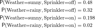
>>> weather = {'Weather':['sunny','rainy']}
>>> sprinkler = {'Sprinkler':['off','on']}
>>> joint = s.Multinom([weather, sprinkler], [0.48, 0.32, 0.198, 0.02])

The list of probabilities is ordered such that the first assignment changes fastest, i.e.

The above approach may work fine for very small models, but becomes unwieldy very quickly when they get larger: for a model of thirty binary-domain variables, we would need a list of probabilities. Therefore, probabilistic models are almost always defined by a factored probability distribution, like:

See also

More about Bayesian networks.

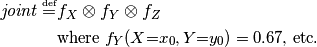
This is an example of a Bayesian network, the most common form of a factored probability distribution, in which there is one factor for each variable (and this factor defines the conditional probabilty distribution over this variable given each assignment to its parents). We could construct this model as follows (given some parameters for the conditional probability distributions):

>>> x = {'X':['x0','x1']}
>>> y = {'Y':['y0','y1']}
>>> z = {'Z':['z0','z1']}
>>> factors = {}    # an empty dictionary which we'll fill with factors
>>> factors['X'] = s.Multinom([x],[0.7,0.3])                  # P(X)
>>> factors['Y'] = s.Multinom([y,x],[0.67,0.33,0.5,0.5])      # P(Y|X)
>>> factors['Z'] = s.Multinom([z,y],[0.1,0.9,0.75,0.25])      # P(Z|Y)
>>> joint = factors['X'].product(factors['Y'], factors['Z'])  # P(X,Y,Z)

The last line is equivalent to the mathematical definition above. It defines joint to be an array of 8 numbers, matched to 8 possible assignments for , and . Each number is a product of three elements: one from each factor array. For example, . symfer knows which element to pick from each array, because the variable names and domains are stored alongside them. In fact, this is such a convenient construction that it is mathematically formalized in Factor algebra (the subject of the next section). To get an idea, in factor algebra the above definition looks like:

But let’s return to handling models. Above, we might as well have introduced a new Python identifier for each factor

>>> p_X = s.Multinom([x],...)
>>> p_Y_given_X = s.Multinom([y,x],...)
>>> p_Z_given_Y = s.Multinom([z,y],...)

but we chose to put them in a dictionary factors instead. This is also the format that symfer uses when loading a model from an external file:

>>> model = s.loadhugin('extended-student.net')
>>> model.keys()
['C', 'D', 'G', 'I', 'H', 'J', 'L', 'S']
>>> model['L']
Multinom(dom=[{'L': ['l0', 'l1']}, {'G': ['g1', 'g2', 'g3']}],par=[0.1, 0.9, 0.4, 0.6, 0.99, 0.01])

See also

The io module contains more functions for loading and saving files.

The model loaded here doesn’t contain an explicit definition of its probability distribution; all inference algorithms implicitly assume that it is the product of the factors. If you would need the joint probability distribution, it is easy enough to define it yourself:

>>> joint = s.I().product(*model.values())
>>> s.evaluate(joint.sumto([]))
Multinom(dom=[],par=[1.0])

In the second line, we check whether it sums to 1 (and according to the output, it does). This is already an example of probabilistic inference, albeit in a very crude way: here, symfer constructs the whole joint distribution, then sums all values. For the reason discussed above, this only works for very small models. Normally you should use an inference algorithm.

To understand how inference algorithms work in symfer, read about Factor algebra.