Factor algebra

In the section Probabilistic models in symfer, we have seen that a model consists of factors: arrays of (usually) probabilities, together with header information (variable names and domains). In this section, we apply operators to these basic factors, thus constructing an an expression in factor algebra.

In symfer this is accomplished using the central data type Factor. To be precise, an instance of (a subclass of) Factor represents a symbolic expression that will evaluate to a factor. For example, in the last three lines of

>>> from symfer import Multinom, SumProd
>>>
>>> weather = {'Weather':['sunny','rainy']}
>>> sprinkler = {'Sprinkler':['off','on']}
>>>
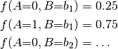
>>> weather_cpd = Multinom([weather],[0.8,0.2])
>>> sprinkler_cpd = Multinom([sprinkler, weather], [0.6,0.4,0.99,0.01] )
>>> joint = SumProd([], [weather_cpd, sprinkler_cpd])

we see three factors being defined; Multinom and SumProd are both Factor subclasses. The Multinom instances are “literal” atomic expressions, where the variables, domains and probabilities are explicitly specified. The SumProd instance is a composite expression, with two operands weather_cpd and sprinkler_cpd which are factor expressions themselves. The SumProd expression signifies that these operands should be multiplied, but the actual multiplication is not performed yet. In effect, as a Python object, a SumProd instance is little more than a container with pointers to the operands.

In parallel to the Python implementation, we also formalize the language of factor expressions in set theory. This formalization may clarify the meaning of the classes, and is also the source of equalities that justify replacing one factor expression with another. We call this formalization factor algebra.

Basic definitions

We assume a set of variables , a set of domains and a function that assigns each variable a domain. A -assignment is a typed function that maps each variable to a value . Here, is a subset of , and is called the assignment domain. An assignment is written using the syntax , which is shorthand for defining function with and values .

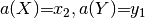Now, a factor on is a typed function from -assignments to numbers. For example, factor could map the assignment to the number . This is also written using a little shorthand:

i.e. the set braces are omitted. With a little abuse of terminology, the assignment domain for factor is also referred to as the factor’s domain, and written . However, keep in mind that when we write this, we formally mean that maps -assignments to numbers.

Note on implementation

Although we have just formally defined factors as functions in set theory, their implementation in symfer has little to do with what a computer scientist or software developer would consider a function. Factors are implemented as arrays, and it is often easier to think of them that way. The array appears when we list all possible assignments and corresponding function values:

assignment	array of function values

This is represented in symfer by storing:

• A Factor attribute domlist == ['X','Y'], listing the variables in in a certain order
• A Factor attribute domtypes, a dict containing and , for example domtypes['X'] == ['x0','x1']
• The array of function values, in the above order (the first variable in domlist changes fastest in the assignment, and its values are enumerated in the order given by domtypes['X']). In Multinom factors, this array is listed in attribute par. In other Factor subclasses, the array is not stored at all, as the Factor merely represents a symbolic expression and not its result. Later, when the symbolic expression is evaluated (during the numeric phase), it is indeed constructed as a native array, which is faster than a Python list. The different evaluators, whose task this is, actually do use the same order.

Operators on factors

An operator we already came across in the introduction at the top of this page is factor multiplication. The product of factor and factor is written , and is itself a factor with domain 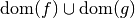. Each of its values is a product of an -value and a -value. For example, if and , then 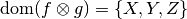, and

It is probably easier to get an idea of factor multiplication in terms of the arrays. Let’s assume that is as shown in the table above, and the array of is like this:

Then the array of is like this:

Note

The arrays are shown two-dimensionally here for legibility. If it were possible, we would have shown both the and arrays two-dimensionally, and the array three-dimensionally, with each dimension matching one variable. As it is, the and variables are collapsed into one dimension.

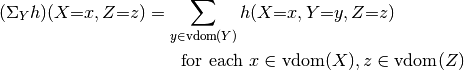
The second important operator is factor summation. This works a little different from normal summation; it does not take two factor operands but only one (let’s say ). The other argument is a set of variables . These variables are summed out of the resulting factor. For example, if and we want to sum out , we write , or actually without the set braces because we are rather lazy than fussy. The resulting factor has and values

Continuing our example, with , the values of are:

These are the most important operators in factor algebra; for the other, we refer to

Sander Evers, Peter J. F. Lucas: Marginalization without Summation: Exploiting Determinism in Factor Algebra. In: Weiru Lu (Ed.), Symbolic and Quantitative Approaches to Reasoning with Uncertainty - 11th European Conference, ECSQARU 2011, Proceedings, pp. 251-262 [SpringerLink] [preprint pdf]

Equalities

The definitions in factor algebra lead to some equalities, which are perhaps not very surprising, but useful to be aware of:

Factor algebra to Factor

Operators in factor algebra correspond to subclasses of Factor. However, this correspondence is not completely one-to-one. The differences are:

• In a Factor, the order of the variables is defined. It is stored in the field domlist.
• Factor sum and product are merged into one operator SumProd. The reason for this is that this operator can be implemented efficiently; the summation is done in-place during the multiplication, so the operator does not require the memory to store the entire product.
• Operands of type Factor are always put in a list (even if there can be only one). This way an expression tree can be traversed in a uniform way. This list is always kept in a field fac.
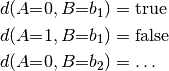
• Similarly, deterministic factor operands (factors with integer values instead of probabilities) are kept in a field det.

A reason for this design is to keep a one-to-one correspondence with the YAML representation. To remove some of the unpracticalities of directly working with this representation, convenience functions are introduced. For example, instead of constructing as symfer.SumProd([],[f,g]) one can also use f.product(g). These convenience functions also behave smart in the sense that they take basic factor algebra simplifications into account. For example, if either f or g is the identity factor I(), product does not return a SumProd expression at all, but simply the other factor.

An overview of available factor algebra operators and their corresponding constructors and convenience functions is shown in the following table.

factor algebra	Factor constructor	Factor convenience function
	SumProd(['A','B'],[f,g])	f.product(g).sumto(['A','B']) or: I().product(f,g).sumto(...)
	f = Multinom([{'A':[0,1]},..], [0.25,0.75,..])
	d = Fun([{'C':[False,True]}], [{'A':[0,1],..], [1,0,..])
	Index([d],[h])	h.index(d)
	Index([Fun([{'C':[False,True]}], [],[1])], [h])	h.index(C=True)
	I()
	Embed([d])	d.embed()
	Reorder([{'newB':'B'}, {'newA':'A'}], [f])	f.reorder([{'newB':'B'}, {'newA':'A'}])